
Guide
A pass through the studio
Eight steps from opening the tool to exporting a review pack, using the model it ships with. Nothing here needs an install. Open the studio in a second tab and follow along.
Four panels and a verdict
The studio opens on a worked example (a roof-mounted autonomy sensor pod) because an empty tool teaches nothing. The window is in four parts. On the left, the assembly tree with each part's mass and a running total. In the centre, the 3D viewport. On the right, a tabbed panel: Properties, Analysis, Trace and BOM. Underneath the viewport, the findings.
The number to look at first is in the toolbar: 7/8 constraints. Seven of the eight executable constraints in this model currently hold. That counter is the tool's one-line verdict, and it updates on every edit.
Start from what is wrong
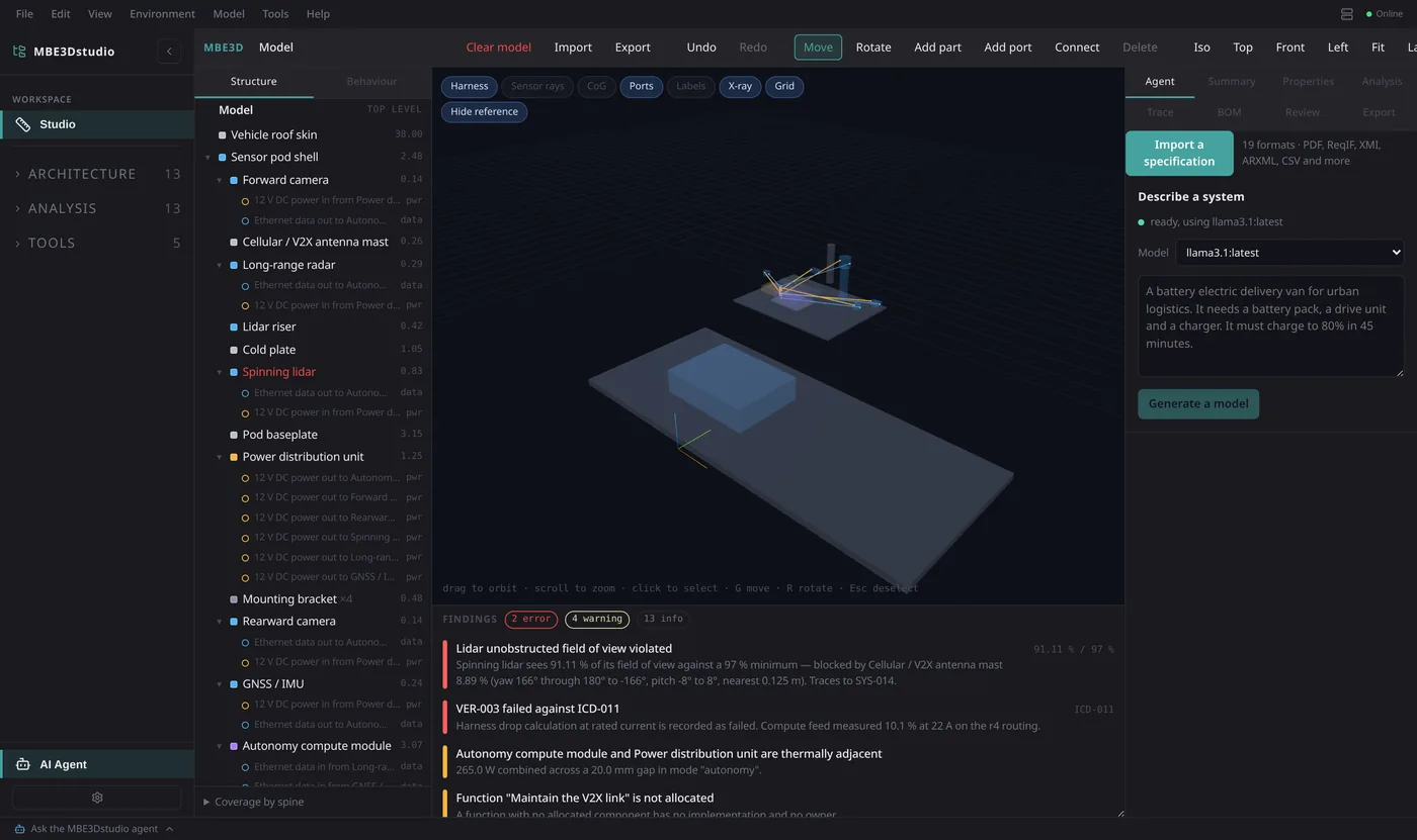
Click a finding rather than a part. Findings are sorted with errors first, and each one names what it measured against what it was allowed. Clicking “Lidar unobstructed field of view violated” selects the spinning lidar and loads it into the inspector.
That is the intended loop: the tool tells you which part has a problem, and selecting the problem selects the part. You can also click parts directly in the tree or in the 3D view, and shift-click to add to the selection.
Everything a part knows
The Properties tab is where a part's real definition lives: its category and parent, its mass, its placement in the parent's frame, its envelope, its power draw for each operating mode, the fraction of that power that becomes heat, and, for a sensor, its field of view, range and boresight.
Two read-only figures sit under the envelope: volume and density. Density is derived from the mass you typed and the envelope you drew. If it comes out at 40 kg/m³ for a machined aluminium bracket, one of those two numbers is wrong, and the tool has just told you so without needing a rule about it.
Move a part and watch the numbers move
Press G for the translate gizmo or R to rotate, then drag. Or type exact coordinates into the placement fields. Both edit the same model, and neither is the “real” one.
Drag the cellular / V2X antenna mast away from the lidar and watch the coverage figure climb past 97 % and the finding disappear mid-drag. The whole analysis pass reruns on every frame of the drag, which is what makes the tool feel like it is arguing with you rather than reporting on you.
Show only what you are working on
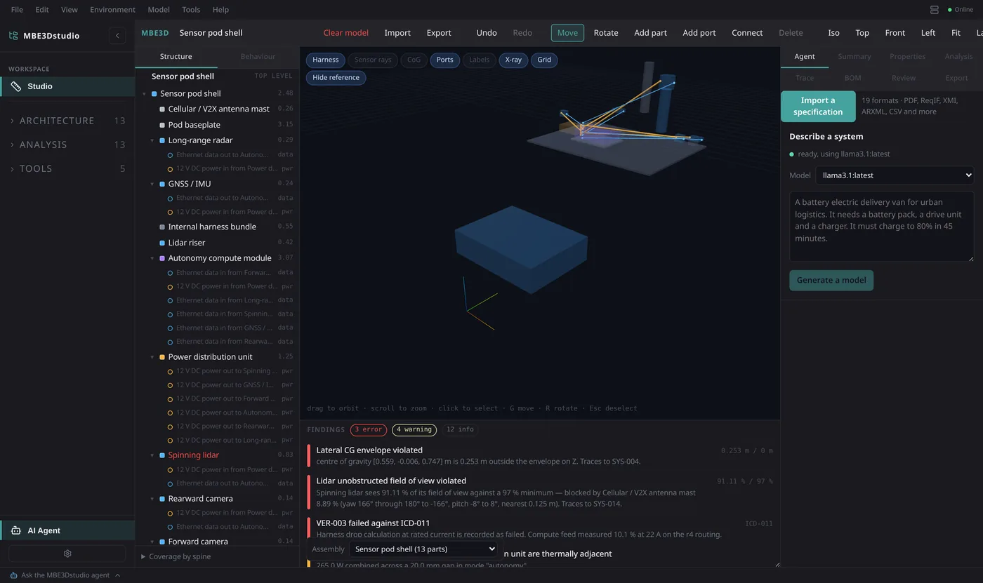
The chips along the top of the viewport control what is drawn: the harness, sensor rays, the centre of gravity marker, ports, labels, the grid, X-ray, interference tinting, and whether the host vehicle is drawn at all.
- X-ray makes envelopes translucent so you can see what is inside the pod shell.
- Sensor rays draws the swept field, colouring rays by whether they reach range or are occluded.
- Hide vehicle drops the reference bodies, useful when the roof skin is in the way, though remember it is still occluding.
- Interference tints overlapping pairs red.
Operating modes are a first-class thing
The mode selector in the toolbar switches which operating mode the power and thermal
numbers are computed for. This model declares three: standby,
nominal and autonomy.
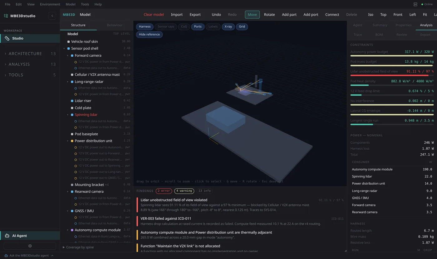
In autonomy this model sits 0.4 W under its 320 W budget. Switch to standby and the roll-up drops from 319.6 W to 43.42 W. That is not the tool being lenient; it is the reason a single worst-case power number is worth so little. The Analysis tab shows all three modes side by side, with the largest consumers ranked for the one you are viewing.
Turn a requirement into a check
A constraint is what makes a requirement enforceable. It has a kind, a limit, a scope and
a unit, and, if you set one, the requirement it came from. Once a constraint names
a requirement, every finding it raises carries that requirement's tag, which is how
“91.11 % against a 97 % minimum” arrives already labelled
SYS-014.
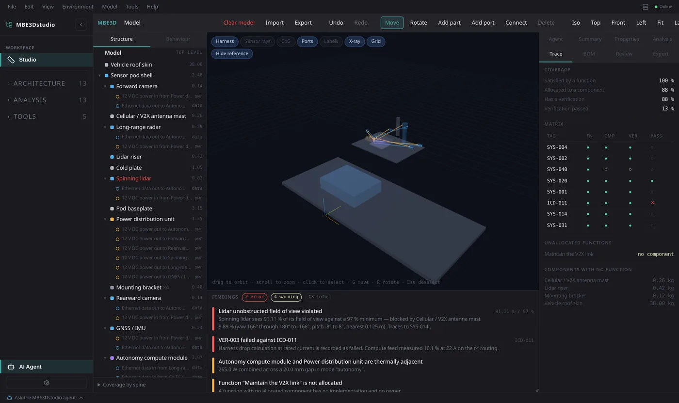
The Trace tab then shows what that buys you: coverage for satisfied, allocated, verified and passing, plus the loose ends: functions allocated to no component, components performing no function. In this model, one function (“Maintain the V2X link”) has no component, and it is listed rather than quietly ignored.
Take it with you
Four buttons on the right of the toolbar. Save writes
the whole project as .mbe.json, the complete description of the work,
because nothing an engineer decides lives outside the model.
Report generates the Markdown review pack.
CSV exports the bill of materials.
PNG captures the viewport as it stands.
The report is built from the same analysis object the screen is showing, so the document you hand a reviewer and the screen you were working on cannot disagree. Your work is also autosaved locally as you go, so closing the tab does not lose it.
| G / R | Translate / rotate gizmo |
| F | Frame the selection |
| Esc | Clear the selection |
| Del | Delete selected parts (children are re-rooted, not deleted) |
| Ctrl+Z / Shift+Ctrl+Z | Undo / redo |
| Ctrl+S | Save the project |